Exponential Random Graph Models

Terms classification for every Exponential Random Graph Model (ERGM)

Terms can be classified in six main ways.

Dyadic independent and dyadic dependent terms: We encounter the first one when the probability of edge formation is related to nodes properties or attributes; we encounter the second when the probability of edge formation depends on other existing edges.
Structural and nodal attributes terms: The first kind provides tools to understand the structure of the network per se; the second kind provides tools to explain how nodal attributes might have influenced the formation of edges.
Terms for directed networks and terms for undirected networks
Exogenous and Endogenous terms: The first one refers to terms using covariates, the second to structural terms.
Markovian or non-Markovian: a Markovian term measures the structure in a network neighborhood
Curved (geometrically weighted ) or non-curved: terms that are tweaked to improve the model stability

Binary Exponential Random Graph Model (ERGM)

An ERGM model is performed through the ergm::ergm function. The basic function call is as follows:

fit <- ergm::ergm(formula)

The formula requires the specification of a network dependent variable, and a list of terms.

Most popular structural/endogenous - dyadic independent terms

edges Extent to which the number of edges in the network characterizes the overall structure (Is it a random number of edges, or it is the meaningful outcome of a certain phenomenon?). Introduces one statistic to the model. Directed and Undirected networks.
density Extent to which the network density characterizes the overall structure (Is it a random density, or it is the meaningful outcome of a certain phenomenon?). Introduces one statistic to the model. Directed and Undirected networks.
sender Extent to which a specific node, compared to a baseline one, is sending out non-random edges (different from the same node’s behavior in a random distribution). Introduces to the model as many statistics as the number of nodes minus one. Directed Networks only.
receiver Extent to which a specific node, compared to a baseline one, is receiving non-random edges (different from the same node’s behavior in a random distribution). Introduces to the model as many statistics as the number of nodes minus one. Directed Networks only.

Most popular structural/endogenous/Markovian - dyadic dependent terms

mutual Extent to which ties are more likely to be reciprocated than they would be in a random network (controlling for the other effects). Introduces one statistic to the model. Directed networks only.
asymmetric Extent to which the observed non reciprocated ties are non-random. Introduces one statistic to the model. Directed networks only.
triangles Extent to which the observed triangles are non-random. Introduces one statistic to the model. Directed and Undirected networks. In the case of directed network measures “transitive triple” and “cyclic triple”, so triangle equals to ttriple plus ctriple.
triadcensus Extent to which the sixteen categories in the categorization of Davis and Leinhardt (1972) are observed in the network and are not generated at random. Introduces 16 statistics to the model. Directed networks only.

Triad Census

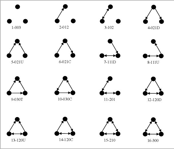
balance Extent to which type 102 or 300 in the categorization of Davis and Leinhardt (1972) -balanced triads- observed in the network are non-random. Introduces one statistic to the model. Directed networks only.
transitive Extent to which type 120D, 030T, 120U, or 300 in the categorization of Davis and Leinhardt (1972) -transitive triads- observed in the network are non-random. Introduces one statistic to the model. Directed networks only.
intransitive Extent to which type 111D, 201, 111U, 021C, or 030C in the categorization of Davis and Leinhardt (1972) -intransitive triads- observed in the network are non-random. Introduces one statistic to the model. Directed networks only.
degree(n), idegree(n), odegree(n) Extent to which nodes with a specified degree are non random. Introduces one statistic to the model. Directed and Undirected networks, with the possibility of in and out specifications for Directed networks.
kstar(n), istar(n), ostar(n) Extent to which stars connecting the specified number of nodes are non random. Introduces one statistic to the model. Directed and Undirected networks, with the possibility of in and out specifications for Directed networks.
cycle(n) Extent to which cycles with a specified number of nodes are non-random. Introduces one statistic to the model. Directed and Undirected networks.

Most popular structural/endogenous/curved - dyadic dependent terms

gwesp(decay=0.25, fixed=FALSE) Geometrically weighted edgewise shared partner distribution. It can be used in place of triangles to improve convergence. The decay parameter should be non-negative. The value supplied for this parameter may be fixed (if fixed=TRUE), or it may be used instead as the starting value for the estimation of decay in a curved exponential family model (when fixed=FALSE, the default) (see Hunter and Handcock, 2006). This term can be used with directed and undirected networks. For directed networks, only outgoing two-path (“OTP”) shared partners are counted.
dgwesp(decay=0.25, fixed=FALSE, type= 'RTP') Geometrically weighted edgewise shared partner distribution. It also counts other types of shared partners not covered by gwesp: Outgoing Two-path (“OTP”), Incoming Two-path (“ITP”), Reciprocated Two-path (“RTP”), Outgoing Shared Partner (“OSP”), Incoming Shared Partner (“ISP”).
gwdegree(decay, fixed=FALSE, attr=NULL, cutoff=30, levels=NULL), gwidegree(.5,fixed=T), gwodegree(.5,fixed=T) Geometrically weighted degree distribution. It can be used in place of degree(n) to improve convergence. Introduces one statistic to the model equal to the weighted degree distribution with decay controlled by the decay parameter. Directed and Undirected networks, with the possibility of in and out specifications for Directed networks.

Most popular nodal covariate terms

nodecov, nodeicov, nodeocov Numeric or Integer attributes. Extent to which the attribute values influence edge formation (same as in a logit model) so that it is non-random under that condition. Introduces one statistic to the model. Directed and Undirected networks, with the possibility of in and out specifications for Directed networks. Dyadic independent.
nodefactor, nodeifactor, nodeofactor Categorical attributes. Extent to which nodes characterized by a specific category form more ties, so that tie formation is non-random under that condition. Introduces to the model a number of statistics equal to the number of categories minus one. Directed and Undirected networks, with the possibility of in and out specifications for Directed networks. Dyadic independent.
absdiff Numeric or Integer attributes. Extent to which common features measured in terms of distance similarity influence edge formation, so that edge formation is non-random under that condition. Introduces one statistic to the model. Directed and Undirected networks. Dyadic independent.
nodematch Categorical attributes. Extent to which nodes characterized by a specific category belonging to a certain attribute form ties with other node characterized by the same category, so that tie formation under that condition is non-random. Introduces to the model as many statistics as the number of categories. Directed and Undirected networks. Dyadic independent. —Differential homophily
edgecov Matrix attribute. Extent to which the ties formed in another context influence tie formation in the context of the current model, so that tie formation under that circumstances is non-random. Introduces one statistic to the model. Directed and Undirected networks. Dyadic dependent.
nodemix Categorical attributes. Extent to which nodes denoted by different categories of an attribute form ties, so that tie formation under these circumstances is non-random. Introduces as many statistics as the number of combinations between every two categories. Directed and Undirected networks. Dyadic independent.

Terms specifications

Use the argument levels within the term specification for selecting the baseline or reference category.

Example: set female as a reference category.

fit <- ergm::ergm(Net ~ edges + nodefactor('sex', levels = -(2)))

Searching for terms

You can look for additional terms with

search.ergmTerms(keyword, net, categories, name)

You have four arguments to help you finding terms:

keyword optional character keyword to search for in the text of the term descriptions. Only matching terms will be returned. Matching is case insensitive.
net a network object that the term would be applied to, used as template to determine directedness, bipartite, etc
categories optional character vector of category tags to use to restrict the results (i.e. ‘curved’, ‘triad-related’) –see categorization of terms in the manual
name optional character name of a specific term to return

Checking your data before the analysis

Before you run any exponential random graph model you must know your data by heart. Not only using descriptive network statistics, but also checking model specifications, before hitting the run button.

Manually check the attribute(s) (numeric, integer, categorical, ordinal)

table(snafun::extract_vertex_attribute(Net, 'sex'))

check mixing of categorical attributes

snafun::make_mixingmatrix(Net, "sex")

check model statistics.

summary(Net ~ edges + nodefactor('sex'))

This last one provides the number of observed cases under the assumptions of each term.

Reading results

You interpret ERGM results as logit models results. Two options:

Compute odd ratios for each coefficient

OR <- exp(coef)

Compute probability for each coefficient

P <- exp(coef) / (1 + exp(coef))

Compute odd ratios using the SNA4DS function


OR <- snafun::stat_ef_int(m)

Compute probability using the snafun function


P <- snafun::stat_ef_int(m, type = "probs")

Simulating networks

It is sometimes helpful to simulate networks with the same features at the one you observed in real life.

Simulating a network from a model

fit <- ergm::ergm(Net ~ edges)
simfit <- simulate(fit, burnin = 1e+6, verbose = TRUE, seed = 9)

simulate network fixing the coefficient results


RandomNet <- network::network(16,density=0.1,directed=FALSE)

sim <- simulate(~ edges + kstar(2), nsim = 2, coef = c(-1.8, 0.03),
                  basis = RandomNet,
                  control = ergm::control.simulate(
                    MCMC.burnin=1000,
                    MCMC.interval=100))
sim[[1]]

MCMC Diagostics

You can check the Monte Carlo Markov Chains diagnostic for your dyadic dependent model using the function:

ergm::mcmc.diagnostics(fit)

Goodness of Fit

You can check the goodness of fit of your model using the function

ergm::gof(fit)

You can also plot your gof output

plot(ergm::gof(fit))

or, making use of your new best friend (the snafun package):

snafun::stat_plot_gof(fit)
stat_plot_gof_as_btergm(fit)

Bipartite ERGMs

A bipartite ERGM works exactly the same way as a binary one. However, in order to make it handle data differentiating between two partitions, it is necessary to use some specially defined terms. Moreover, you will need to specify the model with more advanced settings since it is computationally more demanding.

Importing Bipartite ERGMs

Since you are using the same function as binary ERGM (ergm::ergm) to run the model, it is necessary to make sure that the software knows that it needs to handle a bipartite structure.

Step one: Specify the incidence matrix

The data that contains bipartite network information needs to be specified into a partition 1 X partition 2 data frame or matrix.

If 10 people attend 4 events, the incidence matrix will have dimensions 10 X 4.

Step two: Import the network as a bipartite

You can import the network as bipartite using these specifications.


BipNet <- network::network(BipData, directed = FALSE, bipartite = TRUE)

Step three: Import the attributes

You can import the attributes using this code. The attribute vector needs to contain as many elements as Partition 1 + Partition 2. However, it is unlikely to have an attribute that makes sense for both partitions at the same time.

Make sure to insert the information that concerns partition 1 and afterward the information that concerns partition 2.

Make sure to code as NA the entry for the partition for which you do not have information.

For instance, if we have one attribute for partition one in a network with 10 nodes in partition 1 and 4 in partition 2, we will have the first ten digits storing information about nodes in partition 1 and 4 NAs for partition 2.


# vertex.names <- vector of names
attrib1 <- as.character(c(0, 0, 0, 0, 0, 1, 1, 1, 1, 1, NA, NA, NA, NA))

snafun::add_vertex_attributes(BipNet, "vertex.names",  vertex.names)
snafun::add_vertex_attributes(BipNet, "attrib1",  attrib1)

Step four: Bipartite extra info

In order to make sure that the software correctly reads your bipartite network, you need to code an extra attribute.

The attribute focuses on partition one. For example, if we have 10 nodes in partition 1 we will use:


snafun::add_vertex_attributes(BipNet, "bipratite", value = rep(10, 10), v = 1:10)

Note: bipratite, yes, it is a typo, but a typo in the package. Hence make sure you misspell it; otherwise, you will get an error. (FUN FACT!)

Terms for Bipartite ERGMs

Bipartite ERGMs terms are provided at the same time for both partitions since it is relevant to consider the same structure from both perspectives.

Triad Census

You can find the full list of bipartite terms by running:


ergm::search.ergmTerms(categories = "bipartite")

They are 32 in total, so it is manageable.

The most popular terms are:

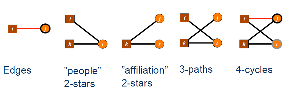
b1star(k) & b2star(k) – star(k) for binary ERGMs
gwb1dsp() & gwb2dsp() – same as gwdsp() for binary ERGMs
b1cov & b2cov – same as nodecov() for binary ERGMs
b1factor & b2factor – same as nodefactor() for binary ERGMs
b1nodematch & b2nodematch – same as nodematch() for binary ERGMs

Specifying advanced options

Since a bipartite ERGM is computationally more demanding than a regular one, you need to make sure you specify the advanced options offered by the ergm package.

Constraints

Constraints are options that allow you to set limits your simulation takes into account

For instance, you can limit the simulation setting a min and a max degree.

constraints= ~ bd(minout = 0, maxout = 7)

For instance,

m <- ergm::ergm(BipNet ~ edges  + b1factor("attr1", levels = -1) + b1star(2),
                 constraints= ~ bd(minout = 0, maxout = 7))

There are many other constraints that it is possible to use

Control

Controls are options that allow you to be aware of what your simulation is doing to a larger extent and, for this reason, to make it faster.

There are several options. For instance,

MCMC.burnin - ignore than many chains before starting to estimate parameters
MCMC.samplesize - collect that number of information from the previous state in order to inform the following one
seed - makes the simulation go the same way every time it is run
MCMLE.maxit - breaks the algorithm after that number of attempts.

For instance,

m <- ergm::ergm(BipNet ~ edges  + b1factor("attr1", levels = -1) + b1star(2),
                 constraints= ~ bd(minout = 0, maxout = 7),
                 control = ergm::control.ergm(MCMC.burnin = 5000,
                                              MCMC.samplesize = 10000,
                                              seed = 1234,
                                              MCMLE.maxit = 20))

Weighted ERGMs

A weighted network is a network where the edges express the weight or the intensity of the relationship.

It is still unimodal, but it contains more information.

In order to use weighted ergms, the network needs to be fully connected.

Different kinds of weights require different models. You need to check:

what kind of variable type characterizes your weights (integer, count, numeric, ordinal…)
what kind of distribution does your weight have

The GERGM package works with fully connected networks and (theoretically ) every kind of weight variable.

The GERGM package does not recognize either the network or the igraph classes.

You need to work with weighted adjacency matrices (NxN - squared, that has inside the weight, rather than 0s and 1s).

Documentation

Installation:

remotes::install_github("matthewjdenny/GERGM", dependencies = TRUE)

User manual

https://github.com/matthewjdenny/GERGM

Vignette

Run browseVignettes("GERGM")in the R console

Running the model

First, we specify the formula,

formula <- adjacencyMatrix ~ edges +
  sender("myCov") +
  receiver("myCov") +
  netcov(otherAdjMat) +
  mutual(alpha = .9)

Then we run the model


set.seed(5)
gergmResults <- GERGM::gergm(formula,
                      estimation_method = "Metropolis", # chose the algorithm to estimate the model
                      covariate_data = covariateData, # passing attributes on
                      number_of_networks_to_simulate = 100000, # same as ergm
                      MCMC_burnin = 10000, # same as ergm
                      thin = 1/10, # retaining only a small number of simulated Networks in the computer memory
                      transformation_type = "Cauchy") # distribution of the weight

The GERGM::gergm function automatically prints results while it runs. However, it is also possible to print them again separately.

Plotting MCMC diagnostics

GERGM::Trace_Plot(gergmResults)

Plotting the Goodnes of fit

GOF(gergmResults)

Plotting the results

GERGM::Estimate_Plot(gergmResults)

Printing a table with standard errors and coefficients

(EstSE <- rbind(t(attributes(gergmResults)$theta.coef),
                t(attributes(gergmResults)$lambda.coef)))

Significance

GERGM models use confidence intervals instead of p-values.

You can estimate the confidence interval using this formula

lower = coef - SE*(-qnorm((1 - 0.95)/2))
upper = coef + SE*(-qnorm((1 - 0.95)/2))

If the lower and the upper intervals are both negative or both positive, the coefficient is significant.

If the lower and the upper intervals have different sign, the coefficient is not significant.