ERGM for temporal networks

The TERGM (=Temporal ERGM) can be used to model a sequence of binary networks. The model is very similar to the ERGM, but the dependent variable is now a list of networks: the first element is the network at time 1, the second element is the network at time 2, et cetera.

How to store the data for a TERGM

You store the data needed for fitting a TERGM as follows.

What	How to store
Time-varying dyadic covariates	Either as a list of networks or matrices
Constant dyadic covariates	Single network or matrix
Vertex level attributes	As vertex attributes inside the observed network objects

How to fit a TERGM

You fit a TERGM with the btergm package (to be installed from CRAN). This fits the model with MPLE, using bootstrapping to derive the standard errors.

The btergm package is compatible with the ergm package and you can use the terms from that package inside btergm.

There are three groups of temporal measures you can specify: memory, delayed reciprocity, and time covariates.

	meaning	btergm
Temporal effects for the ERGM
memory
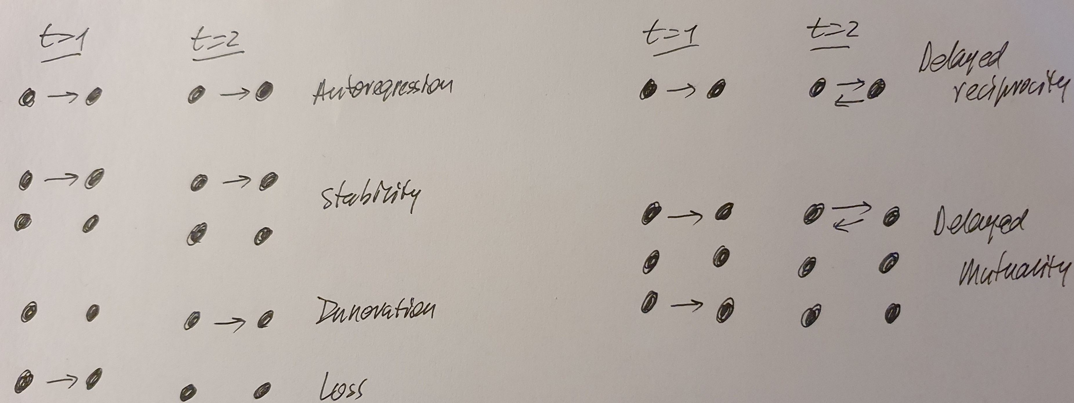
Positive autoregression	Previous existing edges persist in a next network	`btergm::memory(type = "autoregression", lag = 1)`
Dyadic stability	Both previous existing and non-existing ties are carried over to the current network	`btergm::memory(type = "stability", lag = 1)`
Edge innovation	A non-existing previous tie becomes existent in the current network	`btergm::memory(type = "innovation", lag = 1)`
Edge loss	An existing previous tie is dissolved in the current network	`btergm::memory(type = "loss", lag = 1)`
delayed reciprocity
reciprocity	if node j is tied to node i at t = 1, does this lead to a reciprocation of that tie back from i to j at t = 2?	`btergm::delrecip(mutuality = FALSE, lag = 1)`
mutuality	if node j is tied to node i at t = 1, does this lead to a reciprocation of that tie back from i to j at t = 2 AND if i is not tied to j at t = 1, will this lead to j not being tied to i at t = 2? This captures a trend away from asymmetry.	`btergm::delrecip(mutuality = TRUE, lag = 1)`
time covariates
time effect per se	Test for a specific trend (linear or non-linear) for edge formation	`btergm::timecov(transform = function(t) t)`
Time effect of a covariate	Interaction effect to test whether the importance of a covariate increases or decreases over time	`btergm::timecov(x, transform = function(t) t)`

Visually:

TERGM temporal terms

When a timecov is specified without including the value for the transform, the specification defaults to a linear trend over time. For example: timecov() (= the effect of time per se) or timecov(militaryDisputes) (= a linearly increasing or decreasing effect of militaryDisputes over time).

Parallel processing

The btergm package uses MPLE and that lends itself well to parallel processing. You specificy that you want to use parallel processing using the argument parallel.

Windows users can only use parallel = "snow". Other systems can use either parallel = "snow" or parallel = "multicore". The latter is probably often the better choice for non-Windows machines. Both options require that you have the parallel package installed.

If you use the parallel option, you should also specify the appropriate number of cores you want to use. Either set ncpus = 4 (for four cores) or use ncpus = parallel::detectCores() to have R recognize the number of cores automatically (this usually works well, but not always). The ncpus argument is ignored if you do not specify the parallel argument.

The default is no parallel processing.

Goodness-of-fit

Goodness of fit is determined by

gof_m <- btergm:::gof.btergm(m, statistics = btergm_statistics), where

m is a fitted btergm model and btergm_statistics is a vector with statistics to be included in the GoF. The default is

c(btergm::dsp,btergm::esp,btergm::deg,btergm::ideg,btergm::geodesic,btergm::rocpr,btergm::walktrap.modularity).

Of course, the more statistics you include (and the more complex the statistics), the more time it will take for the GoF calculations to finish.

Use ?btergm:::`gof,btergm-method` for more options.

The GoF object can be plotted using btergm:::plot.gof(gof_m) or, often more usefully, through snafun::stat_plot_gof(gof_m). More convenient is to use the helper function from the snafun package. This is:

gof_m <- snafun::stat_plot_gof_as_btergm(m)

By default, this includes the statistics c(btergm::esp, btergm::geodesic, btergm::deg, btergm::rocpr) in the goodness-of-fit, but you can specify other statistics if you prefer. The function returns the goodness-of-fit (in this case, in the gof_m object) and plots it as well. This prevents you from having to use the triple colon ::: for btergm:::gof.btergm and is generally more convenient. If you need the full flexibility of the btergm:::gof.btergm function, use that directly. The results between the two functions are identical.

If you include the btergm::rocpr “statistic” in your GoF, the red line is the Receiver Operating Characteristic (ROC) curve and the blue line is the Precision-Recall curve.

If you see value in the ROC or PR, you can find the arreas under the curves using gof_m$`Tie prediction`$auc.roc and gof_m$`Tie prediction`$auc.pr. Note that Precision-Recall is most appropriate for sparse networks, while ROC works better for more connected networks. Either way, the plots for the network statistics are generally much more informative compared to ROC and PR (because the ROC and PR don’t take the dependency structure in your data into account).

In the other plots, the grey boxplots represent the distribution of the values from the observed networks, the thick black line is the median of the simulations and the dashed line is the mean of the simulations. You can manipulate how each of these are shown by using:

snafun::stat_plot_gof(gof_m, median_include = FALSE, mean_col = "red")

Note: you can also feed a fitted ERGM model to

snafun::snafun::stat_plot_gof_as_btergm(m)

and determine the goodness-of-fit for the fitted ERGM that way.