Temporal networks exploration and description
Source:vignettes/Temporal-networks-exploration.Rmd
Temporal-networks-exploration.RmdTemporal networks (exploration and description)
The main packages to use in this course for descriptive and
exploratory analysis of temporal networks are
networkDynamic to construct and manipulate temporal
networks), tsna (for sna-like network
measures), and ndtv (for visualization).
Edges will typically have a starting time (onset), and
end time (terminus), a duration, a sender
(tail), and a receiver (head). of course,
edges can start and end multiple times during the observation period and
can have durations of length 0 up until any positive number.
The temporal networks are of class networkDynamic.
Network generation and manipulation
-
networkDynamic::networkDynamic: construction of a temporal network. There are many ways in which you can construct a temporal network. A common way is to first construct a network that has the vertex names, any vertex static attributes, edge attributes, whether the network is directed, et cetera.
This network is calledbase.netand is used by this function to extract the basic aspects of the network. Don’t worry that some values (e.g., vertex attributes) may change over time, because any temporal info you add to this function will override what is inbase.net. Butbase.netis an excellent and efficient way to provide much data to the function about the temporal network and it more cumbersome to add that later on.
Further, you can provide dynamic data throughdata.frames for vertices and for edges in several ways. Consult thehelpfunction for the details, as this vignette would become far too long otherwise. -
as.data.frame(g)Extract the dynamic edge info from the network, as adata.frame.
Most of the functions below allow you to specify a time segment you
are interested in. Typically, these include onset,
terminus, length, and at. Below,
we give only one example of how each function can be specified.
networkDynamic::list.vertex.attributes.active(g, onset = 5, terminus = 8)List the attributes of the vertices that are active in a specific time segment.networkDynamic::get.vertex.attribute.active(g, "attrName", at = 1)The value for vertex attributeattrNamein a specific time segment.networkDynamic::list.edge.attributes.active(g, onset = 0, terminus = 49)List the attributes of the edge that are active in a specific time segment.networkDynamic::get.edge.attribute.active(g, "attrName", at = 1)The value for edge attributeattrNamein a specific time segment.networkDynamic::network.extract(classroom, onset = 0, terminus = 1)Extract the part of the temporal network for a specific time segment.networkDynamic::network.collapse(classroom, onset = 0, terminus = 1)Collapse the temporal network into a static network based on the activity within a specific time segment.networkDynamic::activate.vertex.attribute,networkDynamic::activate.edge.attribute,activate.edge.value,activate.network.attributeSet or modify attributes within a specific time segment.deactivate.vertex.attribute,deactivate.edge.attribute,deactivate.network.attributeMake an attribute inactive during a specific time segment.
NOTE: The functions above for accessing and setting the attributes of
a networkDynamic object are not very user friendly.
Luckily, you can also access and/or set attributes using the
network package or the snafun package like in
the network manipulation table. As long as
you want to access and/or set attributes that are static, this
works much easier and uses functions that you have used multiple times
already in this course and should be second nature to you by now.
Network measures and descriptives
networkDynamic::duration.matrix(g, changes, start, end)This function takes a given temporal networkg, a matrix with columns “time”, “tail”, “head” (this matrix is called a toggle list), and a start and end time. It returns adata.framea list of edges and activity spells. A toggle represents a switch from active state to inactive, or vice-versa.network.size(g, onset = 5, length = 10). The size of a network during a specific time segment.
The following functions provide useful descriptives of durations in the temporal network.
tsna::edgeDuration(g, mode = "duration")ortsna::edgeDuration(g, mode = "counts")Sums the activity duration or number of edge events in a time segment.tsna::vertexDuration(g, mode = "duration")ortsna::vertexDuration(g, mode = "counts")Sums the activity duration or number of vertex events in a time segment.tsna::tiedDuration(g, mode = "duration")Measures the total amount of time each vertex has ties.tsna::tiesDuration(g, mode = "counts")Computes the total number of edge spells each vertex is tied by.
The functions tsna::tEdgeFormation and
tsna::tEdgeDissolution compute the number of edges forming
or dissolving at time points over a time segment. If
result.type = 'fraction' the fraction of the number of
edges formed (or dissolved) is computed.
-
tsna::tEdgeFormation(g, start = 1, end = 4, time.interval = 1)Counts at times 1, 2, 3, and 4.
-
tsna::tEdgeDissolution(g, start = 1, end = 4, time.interval = 1)Counts at times 1, 2, 3, and 4.
Calculating measures from sna over time
You can calculate any measure from the sna package on a
collapsed time segment or a series of collapsed time segments through
the tsna::tSnaStats function. These measures can be vertex
level statistics (e.g., sna:betweenness) or graph-level
measures (e.g., sna::grecip). You specify which function
you want to calculate and the time segments they should be calculated
on. The function returns a time series, which makes the outcomes easy to
plot.
For example, you want to calculate transitivity of intervals
that are 5 time points wide. The following function calculates
transitivity for time intervals [0-5), [5-10), [10-15), etc:
tsna::tSnaStats(g, snafun = "gtrans", time.interval = 5, aggregate.dur = 5)
This can cause some sudden shifts of values, so it is often more informative to use overlapping segments. So, let us calculate density for windows of width 0, at intervals of 3. This calculates density for intervals 0-10, 3-13, 6-16, et cetera:
tsna::tSnaStats(g, snafun = "gden", time.interval = 3, aggregate.dur = 10)
Calculating ergm terms over time
The tsna also allows you to compute ergm
terms for specific time segments. Because the model terms provided by
the ergm package (and its various add-ons) are ‘change
statistics’ (that determine the effect of changing a single tie on the
overall network structure), you can use these terms to describe the
network within specific time segments. You specify which terms you want
to calculate using a formula.
For example,
tsna::tErgmStats(g,'~edges + degree(c(1, 2))', start = 3, end = 10)
calculates the number of edges (edges) and the values for
degree(1) and degree(2 for each specified time
segment. The output is a time series (with a column for each statistic)
and can simply be plotted using plot. This plots the time
series for each term above the others, so you can see how all of them
develop over time.
data(windsurfers, package = "networkDynamic")

plot(tsna::tErgmStats(windsurfers,'~edges + degree(2) + kstar(3)',
                      aggregate.dur = 5), main = "ERGM terms over time")
In the lecture, we discussed participation shifts–also known
as p-shifts. Gibson (2003) defined 13 P-shifts, and the
tsna::pShiftCount function can count how often each type
occurs in a specific time segment. This is how Gibson describes each of
the thirteen types:
knitr::include_graphics("pshifts.png")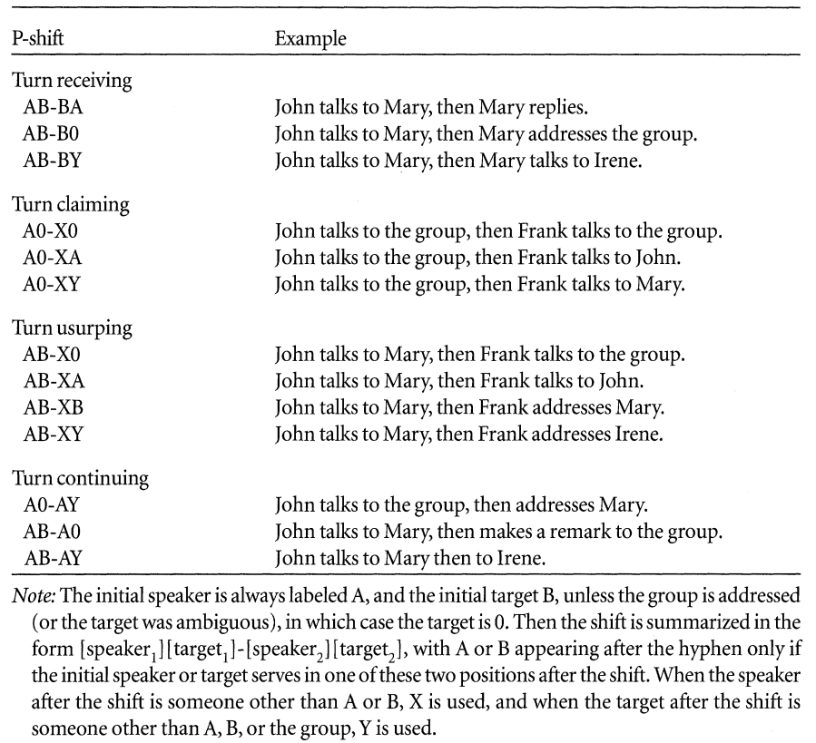
Participation shifts
-
tsna::pShiftCount(g, start = 1, end = 3)Calculates the number of times each of the above P-shifts occurred during the specified time segment. In other words, this calculates the P-shift census.
Temporal paths
The tsna::tPath function calculates the set of
temporally reachable vertices from a given source vertex starting at a
specific time.
-
tsna::tPath(g, v = 12, direction = "fwd", start = 0, end = 3)This calculates the temporal paths from vertex 12 to all other vertices, from the start of the specified time segment. Whendirection = "bkwd", it determines the paths to vertex 12. You can further specify whether you will find the paths that arrive the first or the ones that leave the vertex at the latest possible times.
The generally most relevant parts of the resulting object are:
tdistThe time each specific path takes. When a path does not exist, the value if Inf.gstepsThe length of the path (in terms of the number of steps). When a path does not exist, the value if Inf.
The tsna::plotPaths plots the network and highlights the
calculated temporal paths from the chosen vertex (vertex 12, in the
example above). It can also add a label to each edge, so you can see how
much time it takes for that edge to be activated from this focal vertex.
You can tweak the plot like you would tweak any network plot of class
network.
tsna::plotPaths(
  g,
  paths = tsna::tPath(g, v = 12, direction = "fwd", start = 0, end = 3),
  displaylabels = FALSE,        # remove the vertex labels, to prevent too much visual clutter
  vertex.col = "white",
  edge.label.cex = 1.5          # the color of the printed times
)
A related concept is that of “temporal reachability.” The
tsna::tReach function computes, for each vertex, the number
of vertices that are temporally reachable over the entire observation
period.<> If you want to compute this for a specific time segment,
first use networkDynamic::network.extract to extract the
segment of interest and then feed this to the tsna::tReach
function.
-
tsna::tReach(g, direction = "fwd", start = 10, end = 20)The function to calculate the temporal reachable sets using only temporally forward steps (you can also specifydirection = "bkwd"to determine by how many vertices each vertex can be temporally reached).
Network visualization
Temporal networks can be visualized in two ways. First, static plots can be made of a temporal network, either by collapsing the temporal network into a static network (or to break up the temporal network into static networks of specific time segments).
Visualizing as static networks
An obvious way to visualize the entire temporal network as a static
network is to simply use plot(g).
Alternatively, the temporal network can be collapsed into smaller time segments and plot these the network slices as static representations.
There are two functions that can do this. The ndtv
package has the
ndtv::filmstrip that does this as follows:
-
ndtv::filmstrip(g, frames = 9)This plots the network at 9 points in time. It does not provide an overview of how the network changes over time, but it provides a series of snapshots (9, in this example) of the network. If the timing of the edges is in continuous time, this function has the tendency to plot nearly empty graphs, as it evaluates the networks at specific time points, rather than time intervals.
The snafun package implements a function that divides
the specified time period into time segments of equal time length and
plots each segment as a static network. This is useful to see how the
network changes over time. It also works nicely for networks where
changes happen in continuous time.
snafun::plot_network_slices(9, number = 93)A sometimes useful function is ndtv::proximity.timeline,
which shows the distance between the edges over time. The main purpose
is to see how the edges move vis-a-vis each other over time (based on
the geodesic path distance) and it often helps to see where and when
subgroups are forming over time.
The function call is:
ndtv::proximity.timeline(g,  start = 10, end = 50,
                         time.increment = .5,
                         mode = 'isoMDS')
where you can change the mode to a different scaling algorithm. For actual research projects, you want to try various settings and check which gives you the most informative output for the data at hand.
The function allows you to set many arguments (such as labels and colors).
Visualizing as a dynamic network animation
The ndtv package includes functions to create an
animation of how the network unfolds over time. There are many arguments
you can tweak, so here we only focus on the main approach. Make sure to
consult the package help for more details.
There are two steps in creating a dynamic visualization in
ndtv: you first run ndtv::compute.animation,
which determines coordinates and other aspects of the dynamic plot.
Second, you run ndtv::render.d3movie, which, you guessed
it, renders the actual movie.
# step 0: unfortunately, we have to load the package into our session
library(ndtv)

# step 1: compute the settings
ndtv::compute.animation(g, animation.mode = "kamadakawai",
                        slice.par = list(start = 0, end = 45,
                                         aggregate.dur = 1,
                                         interval = 1, rule = "any"))

# step 2, render the animation
ndtv::render.d3movie(g, usearrows = TRUE, displaylabels = FALSE ,
                     bg = "#111111",
                     edge.col = "#55555599",
                     render.par = list(tween.frames = 15,
                                       show.time = TRUE),
                     d3.options = list(animationDuration = 1000,
                                       playControls = TRUE,
                                       durationControl = TRUE),
                     output.mode = 'htmlWidget'
                     )
Some important arguments for ndtv::render.d3movie
include:
launchBrowser: defaults to TRUE: determines whether the animation will be shown in the Browser after rendering.output.mode: the kind of output you want (defaults to ‘HTML’)filename: The file name of the HTML or JSON file to be generated. Only relevant if you picked ‘HTML’ or ‘JSON’ as output.mode.
Further, you can set most of the common graphical parameters, such as
vertex.col, label.cex,
use.arrows, edge.lwd, et cetera.
If you want to fix vertices to the same location throughout the animation, you do this as follows
# use some way to determine a matrix of vertex locations
coords <- ndtv::network.layout.animate.kamadakawai(g)

# add the x and y coordinates as vertex attributes
# adapt onset and terminus if required
networkDynamic::activate.vertex.attribute(g, "x", coords[, 1],
                                          onset = -Inf, terminus = Inf)

networkDynamic::activate.vertex.attribute(g, "y", coords[, 2],
                                          onset = -Inf, terminus = Inf)

# compute the new animation settings
# We now use `animation.mode = "useAttribute"`
ndtv::compute.animation(g, animation.mode = "useAttribute",
                        slice.par = list(start = 0, end = 45,
                                         aggregate.dur = 1,
                                         interval = 1, rule = "any"))